Excel 2016 Challenges!
Excel Challenge # 1
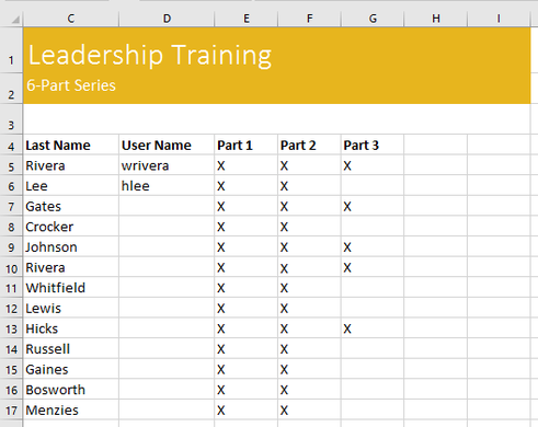
- Open our practice workbook.
- Select cell D6 and type hlee.
- Clear the contents in row 14.
- Delete column G.
- Using either cut and paste or drag and drop, move the contents of row 18 to row 14.
- Use the fill handle to put an X in cells F9:F17.
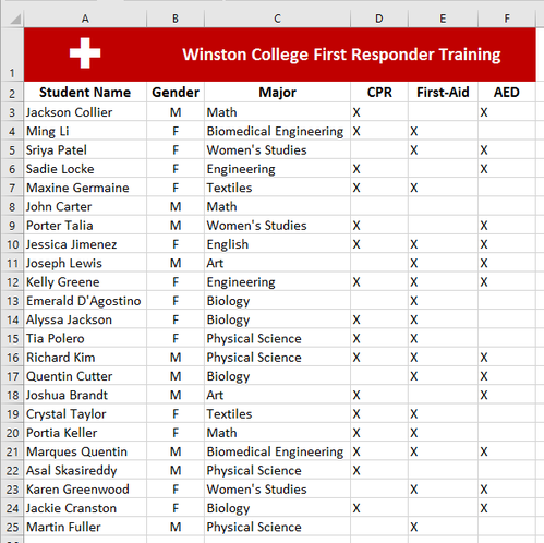
- When you're finished, your workbook should look like this:
- E-mail me your final workbook, titled Challenge #1.
| excel2016_cellbasics_practice__2_.xlsx |
Excel Challenge #2
- Open our practice workbook.
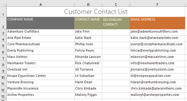
- Autofit Column Width for the entire workbook.
- Modify the row height for rows 3 to 14 to 22.5 (30 pixels).
- Delete row 10.
- Insert a column to the left of column C. Type SECONDARY CONTACT in cell C2.
- Make sure cell C2 is still selected and choose Wrap Text.
- Merge and Center cells A1:F1.
- Hide the Billing Address and Phone columns.
- When you're finished, your workbook should look something like this:
- E-mail me your final workbook, titled Challenge #2.
| excel2016_modifyingcells_practice.xlsx |
Excel Challenge #3
- Open our practice workbook.
- Click the Challenge worksheet tab in the bottom-left of the workbook.
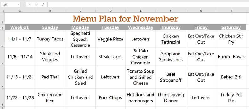
- Change the cell style in cells A2:H2 to Accent 3.
- Change the font size of row 1 to 36 and the font size for the rest of the rows to 18.
- Bold and underline the text in row 2.
- Change the font of row 1 to a font of your choice.
- Change the font of the rest of the rows to a different font of your choice.
- Change the font color of row 1 to a color of your choice.
- Select all of the text in the worksheet, and change the horizontal alignmentto center align and the vertical alignment to middle align.
- When you're finished, your worksheet should look something like this:
- E-mail me your final workbook, titled Challenge #3.
| excel2016_formattingcells_practice.xlsx |
Excel Challenge #4
- Open our practice workbook.
- In cell D2, type today's date and press Enter.
- Click cell D2 and verify that it is using a Date number format. Try changing it to a different date format (for example, Long Date).
- In cell D2, use the Format Cells dialog box to choose the 14-Mar-12 date format.
- Change the sales tax rate in cell D8 to the Percentage format.
- Apply the Currency format to all of column B.
- In cell D8, use the Increase Decimal or Decrease Decimal command to change the number of decimal places to one. It should now display 7.5%.
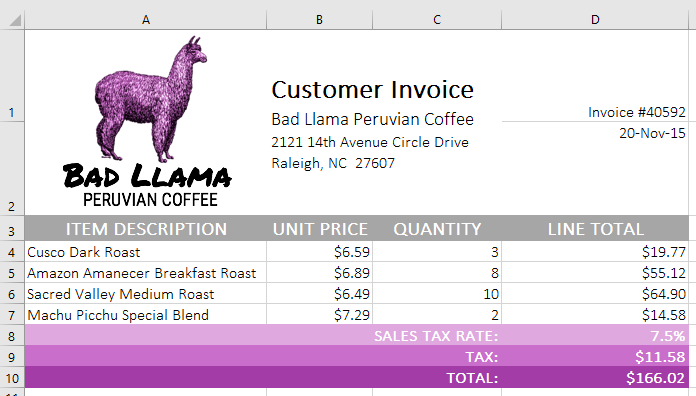
- When you're finished, your spreadsheet should look like this:
| excel2016_numberformats_practice.xlsx |

Excel Challenge #5
- Open our practice workbook.
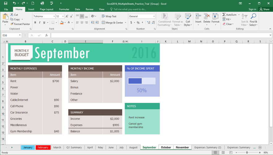
- Insert a new worksheet, and rename it Q1 Summary.
- Move the Expenses Summary worksheet to the far right, then move the Q1 Summary worksheet so that it is between March and April.
- Create a copy of the Expenses Summary worksheet by right-clicking the tab. Do not just copy and paste the content of the worksheet into a new worksheet.
- Change the color of the January tab to blue and the color of the February tab to red.
- Group the worksheets September, October, and November.
- When you're finished, your workbook should look something like this:
| excel2016_multiplesheets_practice.xlsx |
Excel Challenge #6
- Open our practice workbook.
- Click the Challenge tab in the bottom-left of the workbook.
- Crystal Lewis was married and changed her last name to Taylor. Use Find and Replace to change Crystal's last name from Lewis to Taylor. Be careful to onlychange Crystal's last name!
- Find and replace Bio with Biology. Be careful not to change the major Biomedical Engineering!
- Use Find and Replace All to replace the Physics major to Physical Science.
- When you're finished, your worksheet should look like this:
| excel2016_findreplace_practice.xlsx |
Excel Challenge #7
- Open our practice workbook.
- Click the Challenge worksheet tab in the bottom-left of the workbook.
- Run the Spell Check to correct any spelling errors in the workbook.
- Correct the words coffe and medum using the suggested spelling.
- Ignore the spelling suggestion for the word Amanecer.
- When you're finished, your worksheet should look like this below:
- Bonus Step! There is one error Spell Check didn't catch. Can you spot it? Hint:It's in one of the item descriptions.
| excel2016_checkspelling_practice.xlsx |
Excel Challenge #8
- Open our practice workbook.
- Click the East Coast tab at the bottom of the workbook.
- In the Page Layout tab, use the Print Titles feature to repeat row 1 at the top and column A at the left.
- Using the Page Break Preview command, move the break between rows 47 and 48 up so it's between rows 40 and 41.
- In Backstage view, open the Print Pane.
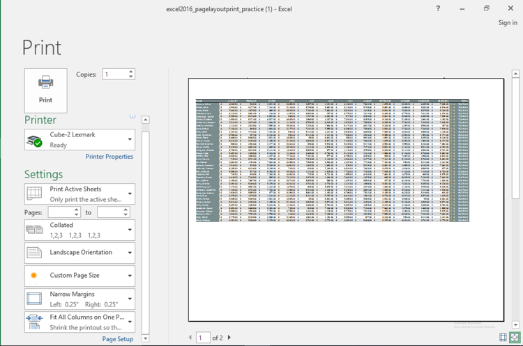
- In the Print pane, change the orientation to Landscape.
- Change the margins to Narrow.
- Change the scaling to Fit All Columns on One Page.
- When you are finished, your print preview should look like this: Include a screen shot of this. Copy and paste.
| excel2016_pagelayoutprint_practice.xlsx |
Excel Challenge #9
- Open our practice workbook.
- Click the Challenge tab in the bottom-left of the workbook.
- Create a formula in cell D4 that multiplies the quantity in B4 by the price per unit in cell C4.
- Use the fill handle to copy the formula in cell D4 to cells D5:D7.
- Change the price per unit for the fried plantains in cell C6 to $2.25. Notice that the line total automatically changes as well.
- Edit the formula for the total in cell D8 so it also adds cell D7.
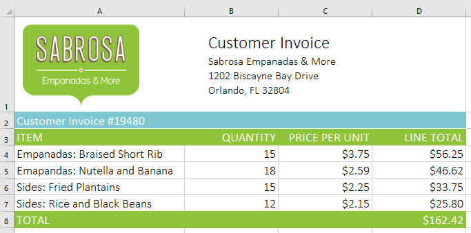
- When you're finished, your workbook should look like this:
| excel2016_introformulas_practice.xlsx |
Excel Challenge #10
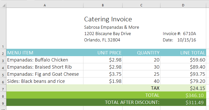
For this challenge, you are going to work with another invoice like the one in our example. In the invoice, you will find the amount of tax for the order, the order's total, and the order's total if you were given a 10% discount.
For this challenge, you are going to work with another invoice like the one in our example. In the invoice, you will find the amount of tax for the order, the order's total, and the order's total if you were given a 10% discount.
- Open our practice workbook.
- Click the Challenge worksheet tab in the bottom-left of the workbook.
- In cell D7, create a formula that calculates the tax for the invoice. Use a sales tax rate of 7.5%.
- In cell D8, create a formula that finds the total for the order. In other words, this formula should add cells D3:D7.
- In cell D9 create a formula that calculates the total after a 10% discount. If you need help understanding how to take a percentage off of a total, check out our lesson on Discounts, Markdowns, and Sales.
- When you're finished, your spreadsheet should look like this:
|
Remember, "The order of operations", Excel calculates formulas based on the following order of operations:
| ||
Excel Challenge #11
- Open our practice workbook.
- Click the Paper Goods tab in the bottom-left of the workbook.
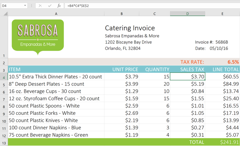
- In cell D4, enter a formula that multiplies the unit price in B4, the quantity in C4, and the tax rate in E2. Make sure to use an absolute cell reference for the tax rate because it will be the same in every cell.
- Use the fill handle to copy the formula you just created to cells D5:D12.
- Change the tax rate in cell E2 to 6.5%. Notice that all of your cells have updated. When you're finished, your workbook should look like this:
| excel2016_cellreferences_practice__3_.xlsx |
6. Click the Catering Invoice tab.
7. Delete the value in cell C5 and replace it with a reference to the total cost of the paper goods. Hint: The cost of
the paper goods is in cell E13 on the Paper Goods worksheet.
7. Delete the value in cell C5 and replace it with a reference to the total cost of the paper goods. Hint: The cost of
the paper goods is in cell E13 on the Paper Goods worksheet.
Excel Challenge #12
- Open our practice workbook.
- Click the Challenge tab in the bottom-left of the workbook.
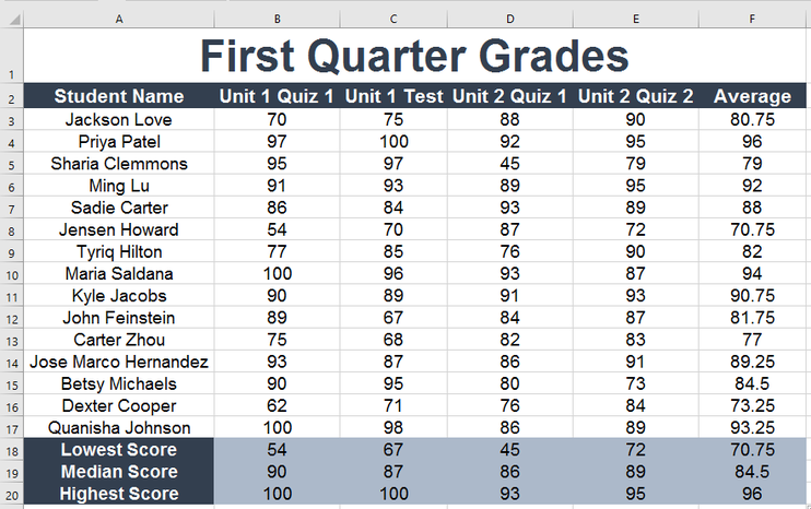
- In cell F3, insert a function to calculate the average of the four scores in cells B3:E3.
- Use the fill handle to copy your function in cell F3 to cells F4:F17.
- In cell B18, use AutoSum to insert a function that calculates the lowest score in cells B3:B17.
- In cell B19, use the Function Library to insert a function that calculates the median of the scores in cells B3:B17. Hint: You can find the median function by going to More Functions > Statistical.
- In cell B20, create a function to calculate the highest score in cells B3:B17.
- Select cells B18:B20, then use the fill handle to copy all three functions you just created to cells C18:F20.
- When you're finished, your workbook should look like this:
| excel2016_functions_practice.xlsx |
Excel Challenge #13
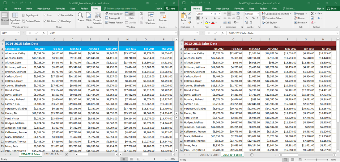
Within our example file, there is A LOT of sales data. For this challenge, we want to be able to compare data for different years side by side. To do this:
Within our example file, there is A LOT of sales data. For this challenge, we want to be able to compare data for different years side by side. To do this:
- Open our practice workbook.
- Open a new window for your workbook.
- Freeze First Column and use the horizontal scroll bar to look at sales from 2015.
- Unfreeze the first column.
- Select cell G17 and click Split to split the worksheet into multiple panes. Hint: This should split the worksheet between rows 16 and 17 and columns F and G.
- Use the horizontal scroll bar in the bottom right of the window to move the worksheet so that Column N, which contains data for January 2015, is next to Column F.
- Open a new window for your workbook, and select the 2012-2013 Sales tab.
- Move your windows so they are side by side. Now you're able to compare data for similar months from several different years. Your screen should look something like this:
| excel2016_freezepanes_practice__4_.xlsx |
Excel Challenge #14
- Open our practice workbook.
- Click the Challenge tab in the bottom-left of the workbook.
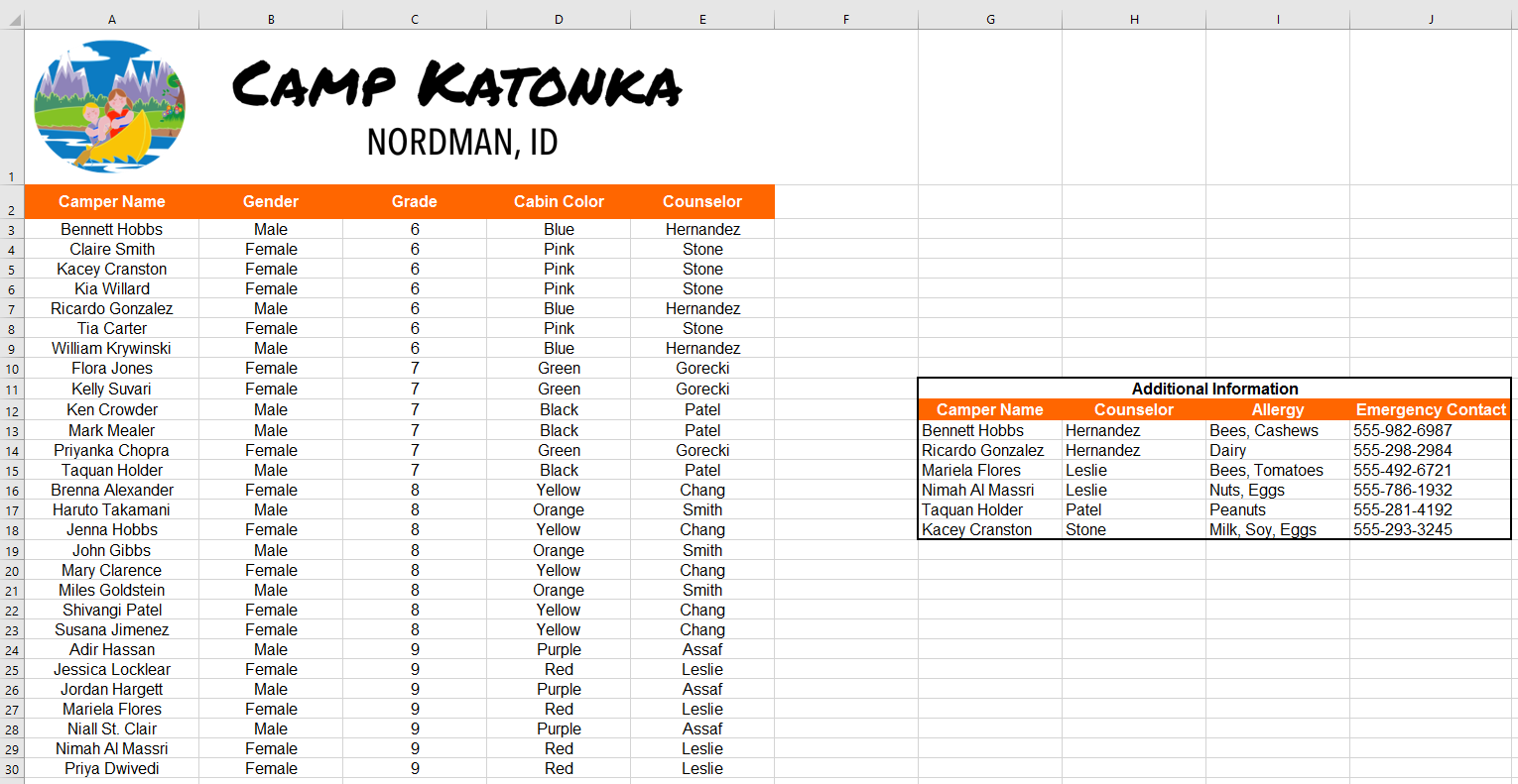
- For the main table, create a custom sort that sorts by Grade from Smallest to Largest and then by Camper Name from A to Z.
- Create a sort for the Additional Information section. Sort by Counselor (Column H) from A to Z.
- When you're finished, your workbook should look like this:
| excel2016_sorting_practice__1_.xlsx |
Excel Challenge # 15
- Open our practice workbook.
- Click the Challenge tab in the bottom-left of the workbook.
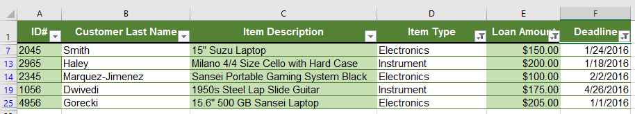
- Apply a filter to show only Electronics and Instruments.
- Use the Search feature to filter item descriptions that contain the word Sansei. After you do this, you should have six entries showing.
- Clear the Item Description filter.
- Using a number filter, show loan amounts greater than or equal to $100.
- Filter to show only items that have deadlines in 2016.
- When you're finished, your workbook should look like this:
| excel2016_filtering_practice.xlsx |
Excel Challenge #16
- Open our practice workbook.
- Click on the Challenge tab in the bottom-left of the workbook.
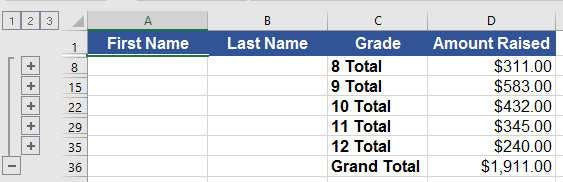
- Sort the workbook by Grade from smallest to largest.
- Use the Subtotal command to group at each change in Grade. Use the SUMfunction and add subtotals to Amount Raised.
- Select Level 2 so that you only see the subtotals and grand total.
- When you're finished, your workbook should look like this:
| excel2016_subtotals_practice.xlsx |
Excel Challenge #17
- Open our practice workbook.
- Click the Challenge tab in the bottom-left of the workbook.
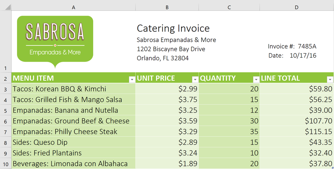
- Select cells A2:D9 and format as table. Choose one of the light styles.
- Insert a row between rows 4 and 5. In the row you just created, type Empanadas: Banana and Nutella, with a unit price of $3.25, and a quantity of 12.
- Change the table style to Table Style Medium 10.
- In Table Style Options, uncheck banded rows and check banded columns.
- When you're finished, your workbook should look like this:
| excel2016_tables_practice__1_.xlsx |
Excel Challenge #18
- Open our practice workbook.
- Click the Challenge tab in the bottom-left of the workbook.
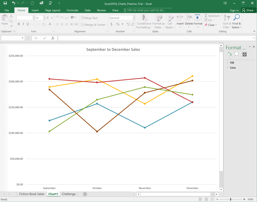
- Select cells A1:E6 and insert a 2D Clustered Column chart.
- Change the chart title to September to December Sales.
- Use the Switch Row/Column command. The columns should now be grouped by month, with a different color for each salesperson.
- Move the chart to a new sheet.
- Change the chart type to line with markers.
- Use the Quick Layout command to change the layout of the chart.
- When you're finished, your workbook should look something like this:
| excel2016_charts_practice.xlsx |
Excel Challenge #19
- Open our practice workbook.
- Click the Challenge worksheet tab in the bottom-left of the workbook.
- Select cells B3:J17.
- Let's say you're the teacher and want to easily see all of the grades that are below passing. Apply Conditional Formatting so it Highlights Cellscontaining values Less Than 70 with a light red fill.
- Now you want to see how the grades compare to each other. Under the Conditional Formatting tab, select the Icon Set called 3 Symbols (Circled). Hint: The names of the icon sets will appear when you hover over them.
- Your spreadsheet should look like this:
| excel2016_conditionalformatting_practice.xlsx |
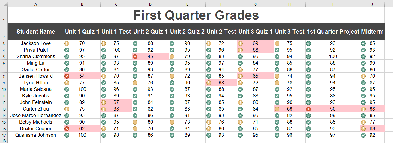
7. Using the Manage Rules feature, remove the light red fill, but keep the icon set.
Excel Challenge # 20
- Open our practice workbook.
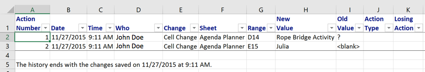
- Turn on Track Changes.
- Replace the value in cell D14 with Rope Bridge Activity.
- Change cell E15 to say Julia.
- Save your workbook.
- List changes on a new sheet. After you do this, the worksheet should look like this:
| excel2016_trackchangescomments_practice__3_.xlsx |
7. Return to the Agenda Planner tab.
8. Add a comment to cell E16 that says snacks will be provided by the exec team.
9. When you're finished, your workbook should look like this:
8. Add a comment to cell E16 that says snacks will be provided by the exec team.
9. When you're finished, your workbook should look like this:
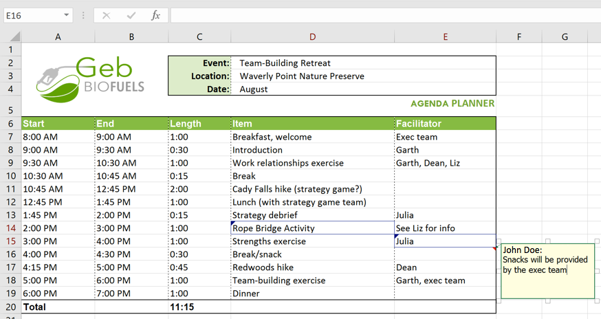
10. Accept All Changes, then turn off Track Changes.
Try to do this on your own, but if you get stuck, see the above link for help. It's supposed to be a challenge.
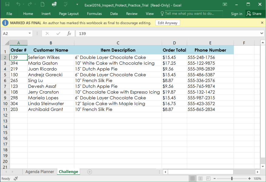
Excel Challenge #21
- Open our practice workbook.
- Use Document Inspector to check the workbook and remove anything it finds.
- Protect the workbook by Marking As Final.
- When you're finished, your workbook should look something like this:
| excel2016_inspectprotect_practice.xlsx |
Try to do this on your own, but if you get stuck, see the above link for help. It's supposed to be a challenge.
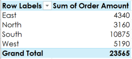
Excel Challenge #22
- Open our practice workbook.
- Create a PivotTable in a separate sheet.
- We want to answer the question What is the total amount sold in each region? To do this, select Region and Order Amount. When you're finished, your workbook should look like this:
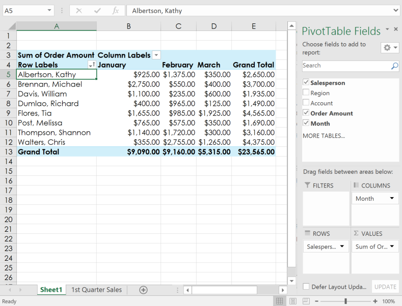
4. In the Rows area, remove Region and replace it with Salesperson.
5. Add Month to the Columns area.
6. Change the number format of cells B5:E13 to Currency. Note: You might have to make columns C and D wider in order to see the values.
7. When you're finished, your workbook should look like this:
5. Add Month to the Columns area.
6. Change the number format of cells B5:E13 to Currency. Note: You might have to make columns C and D wider in order to see the values.
7. When you're finished, your workbook should look like this:
| excel2016_intropivottables_practice.xlsx |
Try to do this on your own, but if you get stuck, see the above link for help. It's supposed to be a challenge.
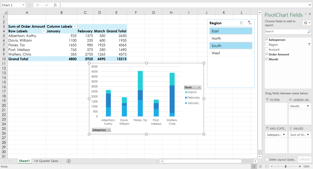
Excel Challenge #23
- Open our practice workbook.
- In the Rows area, remove Region and replace it with Salesperson.
- Insert a PivotChart, and choose the type Line with Markers.
- Insert a slicer for Regions.
- Use the slicer to only show the South and East regions.
- Change the PivotChart type to Stacked Column.
- In the PivotChart Fields pane to the right, add Month to the Legend (Series) area. Note: You can also click the PivotTable and then add Month to the Columns area; the result will be the same.
- When you're finished, your workbook should look something like this:
| excel2016_morepivottables_practice.xlsx |
Try to do this on your own, but if you get stuck, see the above link for help. It's supposed to be a challenge.
Excel Challenge #24
- Open our practice workbook.
- Click the Challenge tab in the bottom-left of the workbook.
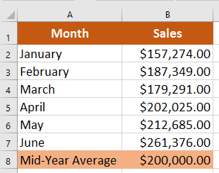
- In cell B8, create a function that calculates the average of the sales in B2:B7.
- The workbook shows Dave's monthly sales amounts for the first half of the year. If he reaches a $200,000 mid-year average, he will receive a 5% bonus. Use Goal Seek to find how much he needs to sell in June in order to make the $200,000 average.
- When you're finished, your workbook should look like this:
| excel2016_whatifanalysis_practice__3_.xlsx |
Try to do this on your own, but if you get stuck, see the above link for help. It's supposed to be a challenge.
Excel Challenge #25
- Open an existing Excel workbook. If you want, you can use our practice workbook.
- Create a simple addition formula using cell references. If you are using the example, create the formula in cell B4 to calculate the total budget.
- Try modifying the value of a cell referenced in a formula. If you are using the example, change the value of cell B2 to $2,000. Notice how the formula in cell B4 recalculates the total.
- Try using the point-and-click method to create a formula. If you are using the example, create a formula in cell G5 that multiplies the cost of napkins by the quantity needed to calculate the total cost.
- Edit a formula using the formula bar. If you are using the example, edit the formula in cell B9 to change the division sign (/) to a minus sign (-).
| excel2013_simpleformulas_practice__3_.xlsx |
Try to do this on your own, but if you get stuck, see the above link for help. It's supposed to be a challenge.
Excel Challenge # 26
- Open an existing Excel workbook. If you want, you can use the example file for this lesson.
- Create a complex formula that will perform addition before multiplication. If you are using the example, create a formula in cell D6 that first adds the values of cells D3, D4, and D5 and then multiplies their total by 0.075. Hint: You'll need to think about the order of operations for this to work correctly.
| complex_formulas_practice.xlsx |
Try to do this on your own, but if you get stuck, see the above link for help. It's supposed to be a challenge.
Excel Challenge #27
- Open an existing Excel workbook. If you want, you can use the example file for this lesson.
- Create a formula that uses a relative reference. If you are using the example, use the fill handle to fill in the formula in cells E4 through E14. Double-click a cell to see the copied formula and the relative cell references.
- Create a formula that uses an absolute reference. If you are using the example, correct the formula in cell D4 to refer only to the tax rate in cell E2 as an absolute reference, then use the fill handle to fill the formula from cells D4 to D14.
- Try referencing a cell across worksheets. If you are using the example, create a cell reference in cell B3 on the Catering Invoice worksheet for cell E15 on the Menu Order worksheet.
| relative_absolute_practice__1_.xlsx |
Try to do this on your own, but if you get stuck, see the above link for help. It's supposed to be a challenge.